[ad_1]
In a earlier tutorial, we’ve explored the usage of the Help Vector Machine algorithm as one of the fashionable supervised machine studying methods that comes applied within the OpenCV library.
To this point, we’ve seen learn how to apply Help Vector Machines to a customized dataset that we’ve generated, consisting of two-dimensional factors gathered into two courses.
On this tutorial, you’re going to learn to apply OpenCV’s Help Vector Machine algorithm to unravel picture classification and detection issues.
After finishing this tutorial, you’ll know:
- A number of of a very powerful traits of Help Vector Machines.
- Easy methods to apply Help Vector Machines to the issues of picture classification and detection.
Let’s get began.

Help Vector Machines for Picture Classification and Detection Utilizing OpenCV
Photograph by Patrick Ryan, some rights reserved.
Tutorial Overview
This tutorial is split into three elements; they’re:
- Recap of How Help Vector Machines Work
- Making use of the SVM Algorithm to Picture Classification
- Making use of the SVM Algorithm to Picture Detection
Recap of How Help Vector Machines Work
In a earlier tutorial, we had been launched to utilizing the Help Vector Machine (SVM) algorithm within the OpenCV library. To this point, we’ve utilized it to a customized dataset that we’ve generated, consisting of two-dimensional factors gathered into two courses.
We have now seen that SVMs search to separate information factors into courses by computing a call boundary that maximizes the margin to the closest information factors from every class, known as the assist vectors. The constraint of maximizing the margin will be relaxed by tuning a parameter known as C, which controls the trade-off between maximizing the margin and lowering the misclassifications on the coaching information.
The SVM algorithm could use completely different kernel features, relying on whether or not the enter information is linearly separable. Within the case of non-linearly separable information, a non-linear kernel could also be used to remodel the information to a higher-dimensional house through which it turns into linearly separable. That is analogous to the SVM discovering a non-linear choice boundary within the unique enter house.
Making use of the SVM Algorithm to Picture Classification
We shall be utilizing the digits dataset in OpenCV for this activity, though the code we’ll develop could also be used with different datasets, too.
Our first step is to load the OpenCV digits picture, divide it into its many sub-images that function handwritten digits from 0 to 9, and create their corresponding floor fact labels that may allow us to quantify the accuracy of the educated SVM classifier later. For this specific instance, we’ll allocate 80% of the dataset pictures to the coaching set, and the remaining 20% of the photographs to the testing set:
|
# Load the digits picture img, sub_imgs = split_images(‘Photographs/digits.png’, 20)
# Acquire coaching and testing datasets from the digits picture digits_train_imgs, digits_train_labels, digits_test_imgs, digits_test_labels = split_data(20, sub_imgs, 0.8) |
Our subsequent step is to create an SVM in OpenCV that makes use of an RBF kernel. As we’ve accomplished in our earlier tutorial, we should set a number of parameter values associated to the SVM sort and the kernel operate in use. We will additionally embody the termination standards to cease the iterative means of the SVM optimization drawback:
|
# Create a brand new SVM svm_digits = ml.SVM_create()
# Set the SVM kernel to RBF svm_digits.setKernel(ml.SVM_RBF) svm_digits.setType(ml.SVM_C_SVC) svm_digits.setGamma(0.5) svm_digits.setC(12) svm_digits.setTermCriteria((TERM_CRITERIA_MAX_ITER + TERM_CRITERIA_EPS, 100, 1e–6)) |
Quite than coaching and testing the SVM on the uncooked picture information, we’ll first convert every picture into its HOG descriptors, as defined in this tutorial. The HOG approach goals for a extra compact illustration of a picture by exploiting its native form and look. Coaching a classifier on HOG descriptors can doubtlessly improve its discriminative energy in distinguishing between completely different courses whereas on the identical time lowering the computational expense of processing the information:
|
# Changing the picture information into HOG descriptors digits_train_hog = hog_descriptors(digits_train_imgs) digits_test_hog = hog_descriptors(digits_test_imgs) |
We could lastly prepare the SVM on the HOG descriptors and proceed to foretell labels for the testing information, primarily based on which we could compute the classifier’s accuracy:
|
# Predict labels for the testing information _, digits_test_pred = svm_digits.predict(digits_test_hog.astype(float32))
# Compute and print the achieved accuracy accuracy_digits = (sum(digits_test_pred.astype(int) == digits_test_labels) / digits_test_labels.dimension) * 100 print(‘Accuracy:’, accuracy_digits[0], ‘%’) |
For this specific instance, the values for C and gamma are being set empirically. Nevertheless, it’s urged {that a} tuning approach, such because the grid search algorithm, is employed to analyze whether or not a greater mixture of hyperparameters can push the classifier’s accuracy even larger.
The entire code itemizing is as follows:
|
1 2 3 4 5 6 7 8 9 10 11 12 13 14 15 16 17 18 19 20 21 22 23 24 25 26 27 28 29 30 31 32 33 34 35 |
from cv2 import ml, TERM_CRITERIA_MAX_ITER, TERM_CRITERIA_EPS from numpy import float32 from digits_dataset import split_images, split_data from feature_extraction import hog_descriptors
# Load the digits picture img, sub_imgs = split_images(‘Photographs/digits.png’, 20)
# Acquire coaching and testing datasets from the digits picture digits_train_imgs, digits_train_labels, digits_test_imgs, digits_test_labels = split_data(20, sub_imgs, 0.8)
# Create a brand new SVM svm_digits = ml.SVM_create()
# Set the SVM kernel to RBF svm_digits.setKernel(ml.SVM_RBF) svm_digits.setType(ml.SVM_C_SVC) svm_digits.setGamma(0.5) svm_digits.setC(12) svm_digits.setTermCriteria((TERM_CRITERIA_MAX_ITER + TERM_CRITERIA_EPS, 100, 1e–6))
# Changing the picture information into HOG descriptors digits_train_hog = hog_descriptors(digits_train_imgs) digits_test_hog = hog_descriptors(digits_test_imgs)
# Practice the SVM on the set of coaching information svm_digits.prepare(digits_train_hog.astype(float32), ml.ROW_SAMPLE, digits_train_labels)
# Predict labels for the testing information _, digits_test_pred = svm_digits.predict(digits_test_hog.astype(float32))
# Compute and print the achieved accuracy accuracy_digits = (sum(digits_test_pred.astype(int) == digits_test_labels) / digits_test_labels.dimension) * 100 print(‘Accuracy:’, accuracy_digits[0], ‘%’) |
Making use of the SVM Algorithm to Picture Detection
It’s potential to increase the concepts we’ve developed above from picture classification to picture detection, the place the latter refers to figuring out and localizing objects of curiosity inside a picture.
We will obtain this by repeating the picture classification we developed within the earlier part at completely different positions inside a bigger picture (we’ll discuss with this bigger picture because the check picture).
For this specific instance, we’ll create a picture that consists of a collage of randomly chosen sub-images from OpenCV’s digits dataset, and we’ll then try to detect any occurrences of a digit of curiosity.
Let’s begin by creating the check picture first. We are going to accomplish that by randomly choosing 25 sub-images equally spaced throughout your entire dataset, shuffling their order, and becoming a member of them collectively right into a $100times 100$-pixel picture:
|
1 2 3 4 5 6 7 8 9 10 11 12 13 14 15 16 17 18 19 20 21 22 23 24 25 26 27 28 29 30 31 32 33 34 35 36 37 38 39 40 41 42 43 44 45 46 |
# Load the digits picture img, sub_imgs = split_images(‘Photographs/digits.png’, 20)
# Acquire coaching and testing datasets from the digits picture digits_train_imgs, _, digits_test_imgs, _ = split_data(20, sub_imgs, 0.8)
# Create an empty record to retailer the random numbers rand_nums = []
# Seed the random quantity generator for repeatability seed(10)
# Select 25 random digits from the testing dataset for i in vary(0, digits_test_imgs.form[0], int(digits_test_imgs.form[0] / 25)):
# Generate a random integer rand = randint(i, int(digits_test_imgs.form[0] / 25) + i – 1)
# Append it to the record rand_nums.append(rand)
# Shuffle the order of the generated random integers shuffle(rand_nums)
# Learn the picture information equivalent to the random integers rand_test_imgs = digits_test_imgs[rand_nums, :]
# Initialize an array to carry the check picture test_img = zeros((100, 100), dtype=uint8)
# Begin a sub-image counter img_count = 0
# Iterate over the check picture for i in vary(0, test_img.form[0], 20): for j in vary(0, test_img.form[1], 20):
# Populate the check picture with the chosen digits test_img[i:i + 20, j:j + 20] = rand_test_imgs[img_count].reshape(20, 20)
# Increment the sub-image counter img_count += 1
# Show the check picture imshow(test_img, cmap=‘grey’) present() |
The ensuing check picture appears as follows:
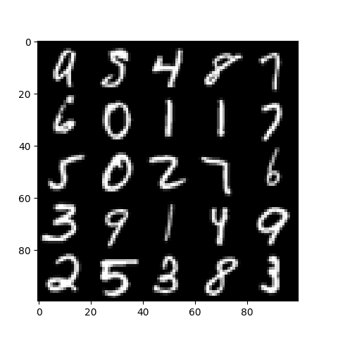
Take a look at Picture for Picture Detection
Subsequent, we will prepare a newly created SVM like what we did within the earlier part. Nevertheless, provided that we are actually addressing a detection drawback, the bottom fact labels shouldn’t correspond to the digits within the pictures; somewhat, they need to distinguish between the constructive and the damaging samples within the coaching set.
Say, as an example, that we’re involved in detecting the 2 occurrences of the 0 digit within the check picture. Therefore, the photographs that includes a 0 within the coaching portion of the dataset are taken to signify the constructive samples and distinguished by a category label of 1. All different pictures belonging to the remaining digits are taken to signify the damaging samples and consequently distinguished by a category label of 0.
As soon as we’ve the bottom fact labels generated, we could proceed to create and prepare an SVM on the coaching dataset:
|
1 2 3 4 5 6 7 8 9 10 11 12 13 14 15 16 17 18 19 |
# Generate labels for the constructive and damaging samples digits_train_labels = ones((digits_train_imgs.form[0], 1), dtype=int) digits_train_labels[int(digits_train_labels.shape[0] / 10):digits_train_labels.form[0], :] = 0
# Create a brand new SVM svm_digits = ml.SVM_create()
# Set the SVM kernel to RBF svm_digits.setKernel(ml.SVM_RBF) svm_digits.setType(ml.SVM_C_SVC) svm_digits.setGamma(0.5) svm_digits.setC(12) svm_digits.setTermCriteria((TERM_CRITERIA_MAX_ITER + TERM_CRITERIA_EPS, 100, 1e–6))
# Convert the coaching pictures to HOG descriptors digits_train_hog = hog_descriptors(digits_train_imgs)
# Practice the SVM on the set of coaching information svm_digits.prepare(digits_train_hog, ml.ROW_SAMPLE, digits_train_labels) |
The ultimate piece of code that we will be including to the code itemizing above performs the next operations:
- Traverses the check picture by a pre-defined stride.
- Crops a picture patch, which is of equal dimension to the sub-images that function the digits (i.e., 20 $instances$ 20 pixels), from the check picture at each iteration.
- Extracts the HOG descriptors of each picture patch.
- Feeds the HOG descriptors into the educated SVM to acquire a label prediction.
- Shops the picture patch coordinates each time a detection is discovered.
- Attracts the bounding field for every detection on the unique check picture.
|
1 2 3 4 5 6 7 8 9 10 11 12 13 14 15 16 17 18 19 20 21 22 23 24 25 26 27 28 29 30 31 32 33 34 35 |
# Create an empty record to retailer the matching patch coordinates positive_patches = []
# Outline the stride to shift with stride = 5
# Iterate over the check picture for i in vary(0, test_img.form[0] – 20 + stride, stride): for j in vary(0, test_img.form[1] – 20 + stride, stride):
# Crop a patch from the check picture patch = test_img[i:i + 20, j:j + 20].reshape(1, 400)
# Convert the picture patch into HOG descriptors patch_hog = hog_descriptors(patch)
# Predict the goal label of the picture patch _, patch_pred = svm_digits.predict(patch_hog.astype(float32))
# If a match is discovered, retailer its coordinate values if patch_pred == 1: positive_patches.append((i, j))
# Convert the record to an array positive_patches = array(positive_patches)
# Iterate over the match coordinates and draw their bounding field for i in vary(positive_patches.form[0]):
rectangle(test_img, (positive_patches[i, 1], positive_patches[i, 0]), (positive_patches[i, 1] + 20, positive_patches[i, 0] + 20), 255, 1)
# Show the check picture imshow(test_img, cmap=‘grey’) present() |
The entire code itemizing is as follows:
|
1 2 3 4 5 6 7 8 9 10 11 12 13 14 15 16 17 18 19 20 21 22 23 24 25 26 27 28 29 30 31 32 33 34 35 36 37 38 39 40 41 42 43 44 45 46 47 48 49 50 51 52 53 54 55 56 57 58 59 60 61 62 63 64 65 66 67 68 69 70 71 72 73 74 75 76 77 78 79 80 81 82 83 84 85 86 87 88 89 90 91 92 93 94 95 96 97 98 99 100 101 102 103 104 105 106 107 108 109 110 |
from cv2 import ml, TERM_CRITERIA_MAX_ITER, TERM_CRITERIA_EPS, rectangle from numpy import float32, zeros, ones, uint8, array from matplotlib.pyplot import imshow, present from digits_dataset import split_images, split_data from feature_extraction import hog_descriptors from random import randint, seed, shuffle
# Load the digits picture img, sub_imgs = split_images(‘Photographs/digits.png’, 20)
# Acquire coaching and testing datasets from the digits picture digits_train_imgs, _, digits_test_imgs, _ = split_data(20, sub_imgs, 0.8)
# Create an empty record to retailer the random numbers rand_nums = []
# Seed the random quantity generator for repeatability seed(10)
# Select 25 random digits from the testing dataset for i in vary(0, digits_test_imgs.form[0], int(digits_test_imgs.form[0] / 25)):
# Generate a random integer rand = randint(i, int(digits_test_imgs.form[0] / 25) + i – 1)
# Append it to the record rand_nums.append(rand)
# Shuffle the order of the generated random integers shuffle(rand_nums)
# Learn the picture information equivalent to the random integers rand_test_imgs = digits_test_imgs[rand_nums, :]
# Initialize an array to carry the check picture test_img = zeros((100, 100), dtype=uint8)
# Begin a sub-image counter img_count = 0
# Iterate over the check picture for i in vary(0, test_img.form[0], 20): for j in vary(0, test_img.form[1], 20):
# Populate the check picture with the chosen digits test_img[i:i + 20, j:j + 20] = rand_test_imgs[img_count].reshape(20, 20)
# Increment the sub-image counter img_count += 1
# Show the check picture imshow(test_img, cmap=‘grey’) present()
# Generate labels for the constructive and damaging samples digits_train_labels = ones((digits_train_imgs.form[0], 1), dtype=int) digits_train_labels[int(digits_train_labels.shape[0] / 10):digits_train_labels.form[0], :] = 0
# Create a brand new SVM svm_digits = ml.SVM_create()
# Set the SVM kernel to RBF svm_digits.setKernel(ml.SVM_RBF) svm_digits.setType(ml.SVM_C_SVC) svm_digits.setGamma(0.5) svm_digits.setC(12) svm_digits.setTermCriteria((TERM_CRITERIA_MAX_ITER + TERM_CRITERIA_EPS, 100, 1e–6))
# Convert the coaching pictures to HOG descriptors digits_train_hog = hog_descriptors(digits_train_imgs)
# Practice the SVM on the set of coaching information svm_digits.prepare(digits_train_hog, ml.ROW_SAMPLE, digits_train_labels)
# Create an empty record to retailer the matching patch coordinates positive_patches = []
# Outline the stride to shift with stride = 5
# Iterate over the check picture for i in vary(0, test_img.form[0] – 20 + stride, stride): for j in vary(0, test_img.form[1] – 20 + stride, stride):
# Crop a patch from the check picture patch = test_img[i:i + 20, j:j + 20].reshape(1, 400)
# Convert the picture patch into HOG descriptors patch_hog = hog_descriptors(patch)
# Predict the goal label of the picture patch _, patch_pred = svm_digits.predict(patch_hog.astype(float32))
# If a match is discovered, retailer its coordinate values if patch_pred == 1: positive_patches.append((i, j))
# Convert the record to an array positive_patches = array(positive_patches)
# Iterate over the match coordinates and draw their bounding field for i in vary(positive_patches.form[0]):
rectangle(test_img, (positive_patches[i, 1], positive_patches[i, 0]), (positive_patches[i, 1] + 20, positive_patches[i, 0] + 20), 255, 1)
# Show the check picture imshow(test_img, cmap=‘grey’) present() |
The ensuing picture exhibits that we’ve efficiently detected the 2 occurrences of the 0 digit within the check picture:
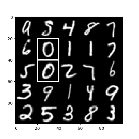
Detecting the Two Occurrences of the 0 Digit
We have now thought of a easy instance, however the identical concepts will be simply tailored to deal with more difficult real-life issues. If you happen to plan to adapt the code above to more difficult issues:
- Keep in mind that the item of curiosity could seem in varied sizes contained in the picture, so that you may want to hold out a multi-scale detection activity.
- Don’t run into the category imbalance drawback when producing constructive and damaging samples to coach your SVM. The examples we’ve thought of on this tutorial had been pictures of little or no variation (we had been restricted to only 10 digits, that includes no variation in scale, lighting, background, and so forth.), and any dataset imbalance appears to have had little or no impact on the detection outcome. Nevertheless, real-life challenges don’t are typically this easy, and an imbalanced distribution between courses can result in poor efficiency.
Additional Studying
This part supplies extra sources on the subject if you wish to go deeper.
Books
Web sites
Abstract
On this tutorial, you discovered learn how to apply OpenCV’s Help Vector Machine algorithm to unravel picture classification and detection issues.
Particularly, you discovered:
- A number of of a very powerful traits of Help Vector Machines.
- Easy methods to apply Help Vector Machines to the issues of picture classification and detection.
Do you’ve gotten any questions?
Ask your questions within the feedback beneath, and I’ll do my finest to reply.
[ad_2]