Unbox the Cox: Intuitive Information to Cox Regressions

[ad_1]

How do hazards and most probability estimates predict occasion rankings?

Introduction

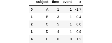
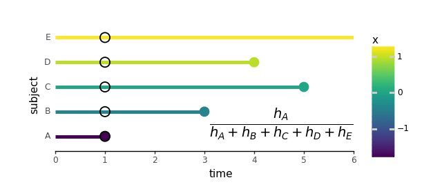
The aim of Cox regression is to mannequin the connection between predictor variables and the time it takes for an occasion to occur — like occasions that solely occur as soon as. Let’s dive right into a made-up dataset with 5 topics, labeled A to E. Through the research, every topic both skilled an occasion (occasion = 1) or not (occasion = 0). On high of that, every topic acquired assigned a single predictor, let’s name it x, earlier than the research. As a sensible instance, if we’re monitoring the dying occasions, then x could possibly be the dosage of a drug we’re testing to see if it helps individuals dwell longer, by affecting the time till dying.

import pandas as pd
import numpy as np

sample_df = pd.DataFrame({
    'topic': ['A', 'B', 'C', 'D', 'E'],
    'time': [1, 3, 5, 4, 6],
    'occasion': [1, 1, 1, 1, 0],
    'x': [-1.7, -0.4, 0.0, 0.9, 1.2],
})

sample_df

On this dataset, topic E didn’t expertise something throughout the research, so we set occasion = 0 and the time assigned is mainly the final second we knew about them. This type of knowledge is named “censored” as a result of we’ve got no clue if the occasion occurred after the research ended. To make it simpler to know, a cool “lollipop” ? plot is useful for visualizing such a knowledge:

from cox.plots import plot_subject_event_times
plot_subject_event_times(sample_df)

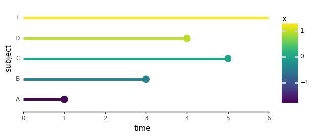
(️️Plotting features out there on my Github repo.)

Only a heads up: I wish to make the principle concepts of Cox regression simpler to know, so we’ll deal with knowledge the place just one occasion can occur at a given time (no ties).

Hazards

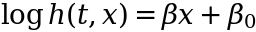
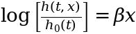
Hazard represents the moment fee (likelihood per unit time) at which an occasion can happen at a selected time — assuming the occasion has not occurred earlier than that time. Since it’s a fee at which occasions happen, it may have arbitrary models and in contrast to likelihood, hazard values can vary between 0 and infinity: [0, ∞).

In Cox regression, hazard works similar to the odds in logistic regression. In logistic regression, odds = p/(1-p) takes probabilities from the range of [0, 1] and transforms them to a spread of [0, ∞). Then, taking the logarithm converts the odds to log-odds, which can have values from negative infinity to positive infinity (-∞, ∞). This log-odds transformation of probabilities is done to match the possible output values to the linear combination of predictors β₁x₁ + β₂x₂ + …, which also can range (-∞, ∞).

Here, we start with a hazard h(t, x) that already has values ranging from 0 to infinity [0, ∞). By applying a logarithm, we transform that range to (-∞, ∞), allowing it to be fitted with a linear combination of predictors:

In Cox regression, there’s another assumption that helps make things easier. It assumes that all the time dependence of the log-hazard is packed into the intercept term:

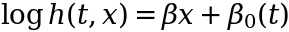
The motivation behind this assumption is to simplify the fitting process significantly (we will show how in a moment). In the literature, the intercept term β₀(t) is usually moved to the left side of this equation and expressed as a baseline hazard log[h₀(t)]:

From this equation, we are able to expressed the hazard h(t, x):

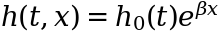
Now, right here is the cool half: because the knowledge from every topic solely involves hazard by predictors x, each topic’s hazard has the identical time dependence. The one distinction lies within the exp(βx) half, which makes hazards from totally different topics proportional to one another. That’s why this mannequin can also be referred to as a “proportional hazard” mannequin.

Now we have been drawing a variety of parallels to the logistic regression. If you happen to learn my earlier submit on logistic regression:

Logistic regression: Faceoff

chances are you’ll be questioning if Cox regression additionally suffers from predictors being “too good”. Keep tuned for the following submit which is able to cowl that!

Likelihoods

Cox fashions are match utilizing a technique referred to as Most Chance Estimation (MLE). Likelihoods are fairly much like chances: they share the identical equation — nearly like two sides of the identical coin. Chances are features of information x, with fastened mannequin parameters βs, whereas likelihoods are features of βs, with fastened x. It‘s like trying on the likelihood density of a Regular distribution, however as an alternative of specializing in x, we deal with μ and σ.

The MLE becoming course of begins with a rank-order of occasion incidence. In our made-up knowledge this order is: A, B, D, C, with E censored. That is the one occasion the place time comes into play in Cox regression. The precise numeric values of occasion occasions don’t matter in any respect, so long as the themes expertise the occasions in the identical order.

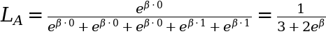
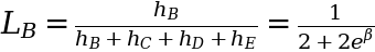
We then transfer on to every topic one after the other and estimate the likelihood or probability of that topic experiencing an occasion in comparison with all the opposite topics who’re nonetheless in danger of getting an occasion. As an illustration, take topic A who skilled an occasion at t = 1. The probability of this occurring is decided by the hazard fee at which topic A experiences the occasion, relative to the mixed hazard charges of everybody else who continues to be in danger at t = 1 (which incorporates everybody):

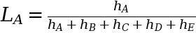
As you’ll have observed, we didn’t trouble defining the baseline hazard h₀(t) as a result of it truly cancels out fully from the probability calculation.

As soon as we substitute the values for x (-1.7, -0.4, 0.0, 0.9, 1.2) for every topic, we find yourself with an equation that solely has β left:

From this level on, for any time after t = 1, the hazard of topic A is taken into account zero and isn’t taken into consideration when calculating additional likelihoods. As an illustration, at one other time, t = 3, topic B experiences an occasion. So, the probability for topic B is decided relative to the hazards of topics B by E solely:

We may preserve going and calculate the likelihoods for all topics A by D, however we’ll cowl that within the coding half within the subsequent part. Topic E, being censored and never experiencing an occasion doesn’t have its personal probability. For the reason that censored knowledge is barely used within the likelihoods of uncensored topics, the ensuing mixed chances are sometimes called “partial probability”.

To summarize this course of, we are able to create an animated lollipop plot:

from cox.plots import animate_subject_event_times_and_mark_at_risk
animate_subject_event_times_and_mark_at_risk(sample_df).save(
    '../pictures/cox_likelihood_fitting_sample.gif'
)

Discovering β

When occasions happen independently of one another, the joint likelihood or probability of observing all occasions may be calculated by multiplying particular person likelihoods, denoted as L= L(A) L(B) L(C) L(D). Nonetheless, multiplying exponential expressions can result in numerical errors, so we regularly take the logarithm of this probability. By making use of the logarithm, we rework the product of likelihoods right into a sum of log-likelihoods:

For the reason that logarithm is a monotonic perform, each the probability and the log-likelihood attain their most level on the identical worth of β. To facilitate visualization and allow comparability with different value features, we are able to outline a price because the damaging log-likelihood and goal to reduce it as an alternative.

Prepared, Set, Code!

We are able to implement this algorithm in Python, step-by-step. First, we have to extract the occasion time and predictor x for every uncensored topic. This may be achieved utilizing the perform event_time_and_x_from_subject(). As soon as we’ve got the occasion time for a topic, we are able to subset our knowledge body to establish the rows comparable to all topics who’re nonetheless in danger. That is achieved utilizing the perform subjects_at_risk_data(). Lastly, we calculate the log-likelihood for every topic utilizing the perform log_likelihood():

def event_time_and_x_from_subject(df, topic):
    subject_with_event_df = df.question(f"topic == '{topic}' & occasion == 1")
    if subject_with_event_df.empty: # Censored topics
        return (np.inf, 0)
    return subject_with_event_df.iloc[0][['time', 'x']]

def subjects_at_risk_data(df, topic):
    time = event_time_and_x_from_subject(df, topic)[0]
    return df.question(f'time >= {time}')

def log_likelihood(df, topic, beta):
    x_subjects_at_risk = subjects_at_risk_data(df, topic)['x']
    x_subject = event_time_and_x_from_subject(df, topic)[1]
    at_risk_hazards = np.exp(beta * x_subjects_at_risk)
    return beta * x_subject - np.log(np.sum(at_risk_hazards))

For visualization functions, we plot the associated fee or damaging log-likelihoods. Subsequently, we have to compute these values for every topic at a selected β worth:

def neg_log_likelihood_for_all_subjects(df, beta):
    topics = df.question("occasion == 1")['subject'].tolist()
    neg_log_likelihoods = [
        -log_likelihood(df, subject, beta)
        for subject in subjects
    ]
    return pd.DataFrame({
        'topic': topics,
        'neg_log_likelihood': neg_log_likelihoods
    })

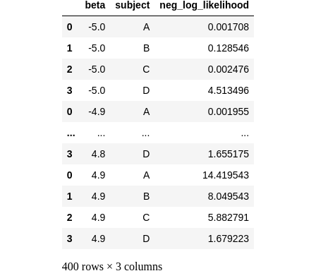
To seek out the minimal value, we sweep by the vary of β values:

def neg_log_likelihood_all_subjects_sweep_betas(df, betas=np.arange(-5, 5, 0.1)):
    loglikelihoods_per_beta = []
    for beta in betas:
        beta_df = neg_log_likelihood_for_all_subjects(df, beta)
        beta_df.insert(0, 'beta', beta) # Add beta column
        loglikelihoods_per_beta.append(beta_df)
    return pd.concat(loglikelihoods_per_beta)

negloglik_sweep_betas_df = neg_log_likelihood_all_subjects_sweep_betas(sample_df)
negloglik_sweep_betas_df

Making sense of it all

Reasonably than aggregating the information body by summing the log-likelihoods grouped by topic, we are able to preserve it in its present type and visualize it as stacked bar charts. On this visualization, the whole peak of every bar corresponds to the sum of damaging log-likelihoods. Every topic is represented by a special colour inside the bar, indicating their particular person probability and contribution to the general probability:

from cox.plots import plot_cost_vs_beta
plot_cost_vs_beta(negloglik_sweep_betas_df, width=0.1)

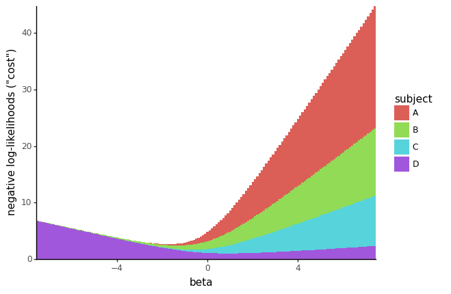
Let’s perceive tips on how to interpret this plot.

First, word that the damaging log-likelihood (value) is massive when the probability and hazards are small. Consider the y-axis much like -log(p-value); bigger values point out decrease likelihood.

Second, censored topics (like topic E) don’t have their very own particular person likelihoods, in order that they don’t seem on the plot. Nonetheless, their contribution is integrated into the likelihoods of topics A to D.

Now, take into account totally different eventualities primarily based on the worth of β:

• If β is massive and damaging, topics A, B, and C (with x ≤ 0) and their occasions are fitted practically completely. The likelihoods of those topics are all shut to 1. Nonetheless, becoming such massive damaging β values for A, B, and C comes at the price of topic D. On this vary of β, the likelihood of topic D (with x > 0) having an occasion could be very low. Because of this, the whole value is dominated by the small probability of topic D.
• If β is massive and constructive, the hazard of topic D (with x > 0) turns into important in comparison with the opposite hazards. The purple part (topic D) turns into a small a part of the whole value. Nonetheless, since topics A, B, and C all have x ≤ 0, the price of becoming a big β for them is excessive. Consequently, these topics dominate the whole value.
• The optimum worth of β, situated round 2 on the plot, strikes a steadiness between assigning excessive chances to occasions of topics A, B, and C versus topic D. This optimum worth may be verified numerically:

negloglik_sweep_betas_df 
    .groupby("beta") 
    .agg(sum_neg_log_likelihood=('neg_log_likelihood', 'sum')) 
    .reset_index() 
    .sort_values('sum_neg_log_likelihood') 
    .head(1)

Utilizing lifelines library

Now that we’ve got a greater understanding of how Cox regression works, we are able to apply it to pattern knowledge utilizing Python’s lifelines library to confirm the outcomes. Here’s a code snippet for our made-up knowledge:

from lifelines import CoxPHFitter

sample_cox_model = CoxPHFitter()
sample_cox_model.match(sample_df, duration_col='time', event_col='occasion', formulation='x')
sample_cox_model.print_summary()

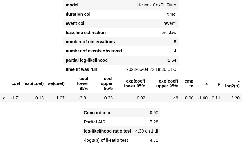
Within the output, we are able to observe the coefficient (coef) worth of -1.71, which corresponds to the β coefficient. Subsequent to it, we’ve got exp(coef), representing exp(β), in addition to columns indicating commonplace errors and confidence intervals. The “partial log-likelihood” worth is -2.64, which matches our handbook end result.

Lastly, you will need to point out that Cox regression implementations additionally provide an extension that permits the mannequin to deal with a number of occasions tied on the identical occasion time. Nonetheless, this goes past the scope of this dialogue.

Conclusion

There was rather a lot to “unbox” right here:

• Cox regression fashions the affiliation between predictor variables and the rank-order of occasions to an occasion incidence.
• Precise numeric values of occasion occasions don’t matter in any respect, so long as the themes expertise the occasions in the identical order.
• Hazards are chances per unit time and may have arbitrary models, whereas likelihoods are associated the likelihood of occasions occurring.
• Stacked bar charts can be utilized to offer insights into most probability estimation by stacking particular person damaging log-likelihoods and exploring how they alter with predictors x.
• By hanging a steadiness between assigning chances to occasions for varied topics, MLE finds β for which the noticed knowledge is more than likely to occur.

To be continued… ?

References

• Code with plots: https://github.com/igor-sb/weblog/blob/essential/posts/cox/plots.py
• Survival Knowledge Evaluation slides from Prof. Patrick Breheny: https://myweb.uiowa.edu/pbreheny/7210/f19/index.html
• ChatGPT for textual content cleanup and humorous hallucinations

---

Unbox the Cox: Intuitive Information to Cox Regressions was initially printed in In the direction of Knowledge Science on Medium, the place individuals are persevering with the dialog by highlighting and responding to this story.

[ad_2]